Surveying with the Total Station: Creating a Micro/Meso Topography of Campus

Introduction

Continuing on with surveying methods, this week's lab focused on collecting data with x, y, and z coordinates. Working in small groups of three, we were given the task of surveying out the micro/meso topography of a one hectare plot area. This was done using a Topcon total station blue toothed to a GMS-2 GPS.

Study Area - For this project our study area was a hectare (100 meters x 100 meters) plot located in the campus mall area of UW-Eau Claire. Most of the study area was uniform in flatness, with a general sloping trend towards the stream which runs almost parallel to the path between flags 2 and 3, shown in figure 1. The area around the stream had a much greater slope which will be evident by the DEM images created in ArcScene, shown later in the report.

Figure 1. This panorama was taken from the corner of an approximately square hectare area. The study area,
highlighted in yellow, is located on the University of Wisconsin - Eau Claire campus mall area. The blue arrow
shows the occupied point where all the points were surveyed from with the total station. The orange arrow,
just to the left of the bridge, shows the location of the back sight used to orient the total station.

Methods

Figure 2 Shows how to collect a
point with the Total Station. One
operator will look through the lens
of the Total Station aiming the
crosshairs in the center of the prism
on the top of the pole. The other person
will try to remain as motionless as possible.
Once the point is "shot" the pole person
moves to the next point.

I have a more detailed step by step walk through of the total station on my "how to" blog. However, I have listed a VERY generalized process below.
1) Set up the Total Station....secure tripod into the ground, use the proper levels the balance the system.
2) Set up the Blue Tooth from GPS to Total Station.
3) Set up a TopSurv Job.
4) Collect GPS points
5) Set your occupied point and your backsight
6) Collect Data
7) Export points to a shapefile from TopSurv using Active Sync.
The exported file will be in a text format. Before a shapefile can be created the text file had to be opened up and edited.

Header>>Delimiter(,)FileFormat(Name,Lat(North), Lon(East),Ht(G),Codes)<<

The highlighted portions need to be deleted. After edited, the file can be exported as a text format in comma delineated format. From here the file can be converted into a shapefile. Figure 3 shows the results of the total station after the shapefile was created.

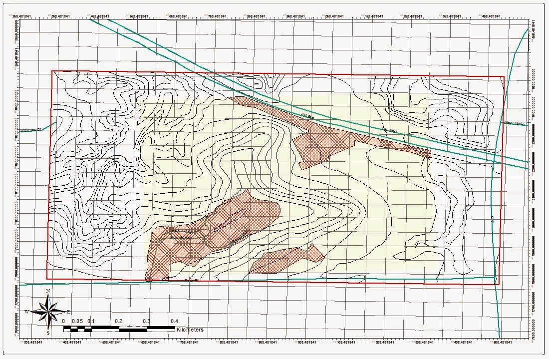
Figure 3 shows the one hectre plot of land we surveyed with the Total Station. As you can see the UW-Eau Claire campus has changed recently, we surveyed in the middle of the green space shown in figure 1. 

Once the elevation points were added to ArcMap, Kriging (3D Analyist) was used to create a elevation surface. The decision to use Kriging to create the surface was based off my analysis during a previous lab which analyzed the various types of interpolation methods: IDW, Natural Neighbor, Spline, and Kriging. My main decision to use Kriging was because it created a new surface and created new values even where data was not collected. Kriging creates the new surface based off the first rule of geography, assuming that closer points are more closely related than those farther away. Figure 4 shows the results of my group's kriging surface from the surveyed data.

Figure 4 shows the resulting kriging surface from the Total Station survey. Over 130 points were collected over this one hectre area. More points were collected over area's with high slope, all of which were along the river. The elevation change from this model was just under five meters.

Once the surface model was created for my group, the other groups survey models were added to ArcScene. Although each group had to survey a one hectare area on the campus mall, not all surveyed the exact same location. Even with the slight differences in the area surveyed you can still see the differences in elevation that the survey's recorded, figures 5 and 6 show just how well the survey's match up.

Figure 5 shows five of the groups in Field Methods all overlayed on top of one another. For a better
analysis of the area I have created some landmark features giving clues to the elevation changes on the
kriging models. The bridge over the Little Niagra creek was difficult to shoot and may look different if
more points were collected closer to the base of the bridge. Also take note in the gaps between the surfaces.
There was over eight meters between the lowest values in group 2 and those of group 6. The color scale on
the top of figure 5 is only applicable to the top layer of group 2. 

Figure 6 shows a view point almost looking almost parallel to the ground. This viewpoint better illustrates the differences in elevation between the five group's layers. Groups 1, 3, and 4 had similar elevation values; meanwhile, groups 2 and 6 were outliers, sitting either significantly lower or higher, respectively. This discrepancy likely is the result from the inaccuracies of the GPS unit used to collect the occupied point for the Total Station. This goes to show ho the accuracy of the survey, with the Total Station, is only as accurate as the GPS used to collect the occupied point.

Discussion

Most of the difficulties with this lab came during the initial setup phase, specifically when trying to set the back sight. We had briefly been instructed on the basics of the total station; which included, set up of the total station for both the physical assembly and leveling of the station as well as the technical steps necessary before surveying can begin. However, we lacked the hands on experience of operating the total station, which resulted in amateur mistakes. When we tried to set the back sight for the total station to orient north with, we made the mistake of having the lens flipped in the wrong direction. We thought since the knobs could be used to precisely move the lens that they should be facing towards you. It was not until 2 hours of trouble shooting that we finally called it a day and had to try again over the weekend after we had found the error in our methods.

Additional difficulties came with trying to accurately capture the elevation changes along the river. One of the problems arose with a broken knob on the pole which raised and lowered the height of the prism. It was set at 2 meters, so this wasn't a major concern. However, if the knob was intact we would have raised the prism higher when we were surveying behind the bridge. There were a few spots along the stream just behind the bridge that we decided to skip because we didn't find it necessary to move the total station to collect two or three more points. Also, just having a varied surface was a difficult trade off. Since we had never used the total station to collect elevation we were not sure of how many points would be necessary to accurately portray the elevation changes. We did take more readings along the river, where the most severe elevation changes were found.

In addition to individual group struggles, there is also the issue of accuracy that comes with the GPS. The Total Station itself is extremely accurate. However, the Total Station has to be given an occupy point. This occupy point is the reference point for all other points in the survey; unless the total station is moved, then the new occupy point will act as the reference point. So although each group may have followed similar procedures and surveyed a relatively similar area, the GPS gave different reference heights for each survey and as a result the kriging surfaces don't match up, in regards to elevation.

Conclusion

Surveying with the Total Station was an effective experience into another important method of data collection. Prior to this I had only used a GPS to collect data. Once the Total Station was set up, the actual surveying went much faster than using a GPS; also, the Total Station was much more consistent. With a GPS you can get high PDOP values behind buildings and your data will be skewed. With the Total Station, there is likely only a handful of GPS points you will ever need to collect, lessening the chance of multipath effects on the GPS signal. In the future I hope I have the opportunity to use a Total Station again, but with a more accurate GPS at the survey grade level.

Priory Navigation 1: Creating a Field Navigation Map and Distance/Bearing Navigation

Introduction

Navigating during field work is of the utmost importance. Whether you are surveying the land for a future building or trekking through the forest on vacation, knowing your location is important. With the invention of GPS, navigation has become increasingly simple, to the point where novice navigators can rely on the GPS to take them wherever they need to be. The problem with this heavy dependence on technology is when it fails. Even a top of the line GPS will give extremely inaccurate data or fail altogether in thick foliage, in/and around buildings, hilly regions, etc.. This is why the effective use of map and compass becomes so important. With this idea of 'low tech' skills, this lab will focus on designing an effective map for navigating a UW-Eau Claire property just south the campus.

The navigation of the course will be two part. The first excursion will be a race to see which group, of three, can complete the course the fastest using only a map and compass. The second day on the course will have the same goal, but each member of the group will be equipped with a GPS and paintball guns. If hit, the group will have to pause for 30 seconds before they can continue on in their navigation. This will test the diligence of the group and the quick thinking navigation in the event of obstacles.

Just like loading a data dictionary in a GPS, too much information on a map will slow you down. Added elements will make essential elements difficult to interpret; and, a constant coverage of ink on the map, maybe from an aerial photo, will make field notes difficult to add. In order to make the best map careful thought about the exercise was needed.

Since we will be using pace count--a technique of counting steps and interpolating the number of those steps to a distance, usually a standard number of steps per 100 meters-- to measure our distance, it will be important to know the topology of the area. Specifically, knowing where steep hillsides are, if there are lowland areas which could create swampy conditions during the winter thaw, etc. Other factors that would be helpful would be landmarks. These landmarks could be used to orient yourself with the proper azimuth calculations. Unfortunately, there are only a couple buildings on the property, and there will be dense foliage blocking these buildings from view. For this purpose I chose to exclude buildings from my map in order to cut down the the clutter. In the end I chose to include:

• 5 meter Contour Lines, with labels
• Navigational Boundaries
• No shooting zones
• Flag Boundaries
• Roads
• A grid overlay (added in layout view)

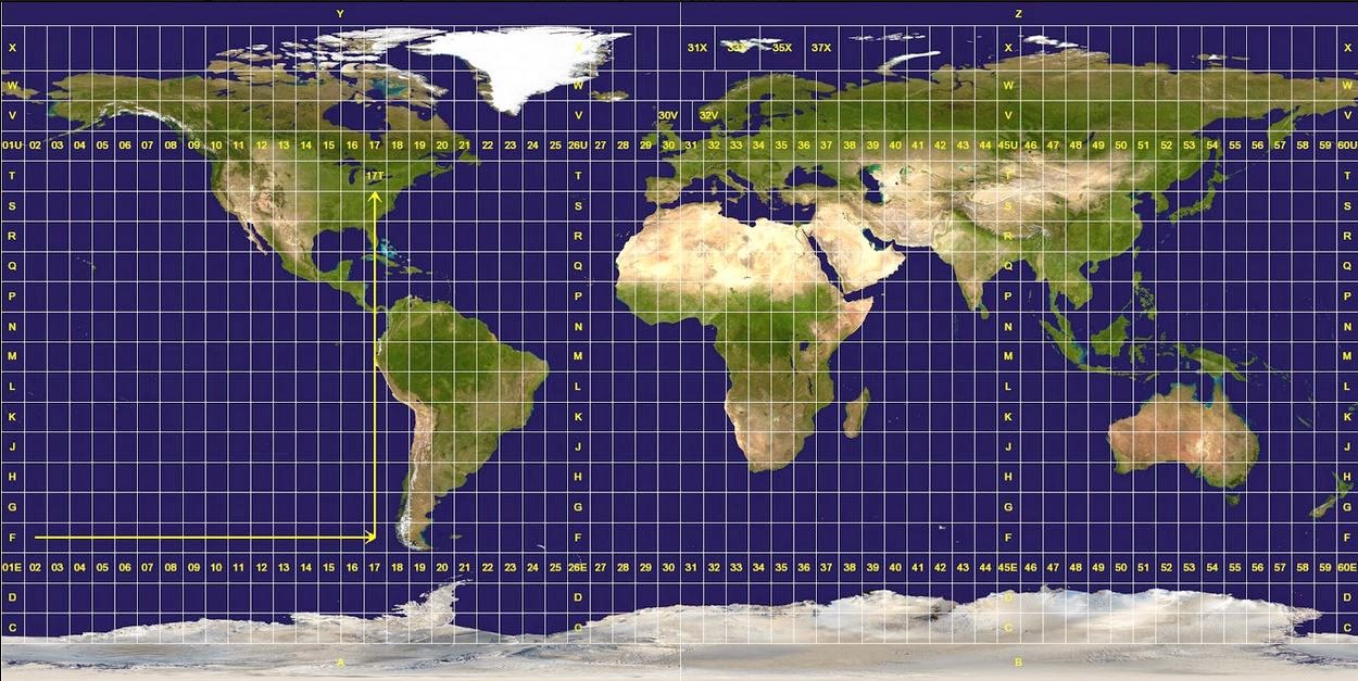
The final requirement is unique to this exercise. In order to familiarize ourselves with different units and coordinate systems, the professor made a requirement that we use a grid based off meters and another off decimal degrees. The map with the meter grid will be projected using the UTM coordinate system while the other will be projected using the Geographic Coordinate System. Shown below in figure 1, the Universal Transverse Mercator coordinate system (UTM) divides the earth into 60 zones, each in six-degree bands of longitude. It is projected using a transverse Mercator projection. The Geographic Coordinate System is based off of a spherical representation and uses latitude and longitude for location purposes.

Figure 1 shows the world divided up in the 60 zones of the UTM coordinate system. The Universal Transverse Mercator coordinate system is projected using a transverse Mercator projection.

Methods

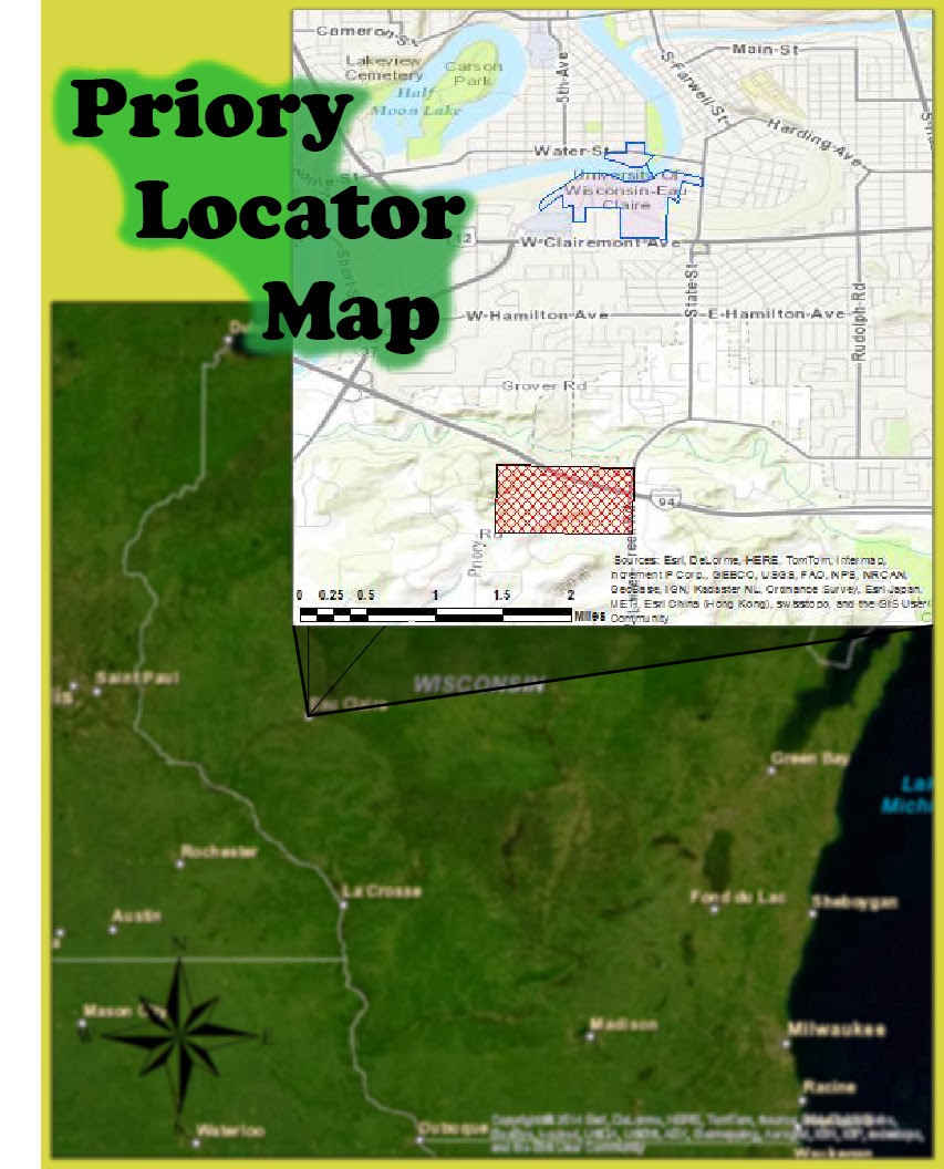
Figure 2 Shows the location of the Priory (red),
three miles south of the UW-Eau Claire campus
(blue). The Priory is a 112 acre parcel of land
consisting mostly of wooded land with three
building complexes. The Priory was acquired
in 2011, and loaned to UW-Eau Claire for
the next 15 years.

This map is part of a larger activity where the class will go out into the field and navigate a course located at the Priory. The Priory is a 112-acre parcel of land consisting of mostly wooded acres in the town of Washington, which is located three miles south of the UW-Eau Claire campus, Figure 2 shows its general whereabouts. The Priory also contains three building complexes totaling approximately 80,000 square feet; however, for our purposes the building's will only serve as areas to be avoided.

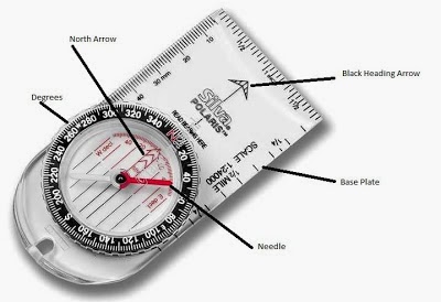
For the actual activity we will us a map and compass to navigate the course. These tools will be essential to the method of distance/azimuth navigation (azimuth is referring to the angular measurement in a spherical coordinate system; on a compass it would refer to the degrees from magnetic north). Essentially if you know your location, you can use an angle with a distance to find another point. The map is used to find your location/the location of the place you want to be; and, the distance/azimuth can be interpolated from the map. Figure 3 shows an image of the compasses we used during our navigation, as well as some of the components on the compass.

Figure 3. A common type of compass for its low cost and easy to use features. Some of the important features to identify are the heading arrow, which indicate your direction of travel. Also note the red arrow inside the compass dial which points to the red "N". This can be used in finding a bearing or, for more general purposes, to find north. The dial is final important aspect of the compass. The dial can twisted and, with the proper knowledge, used to find a bearing.

Basics of Finding/Following a Bearing:

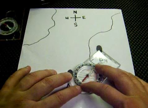
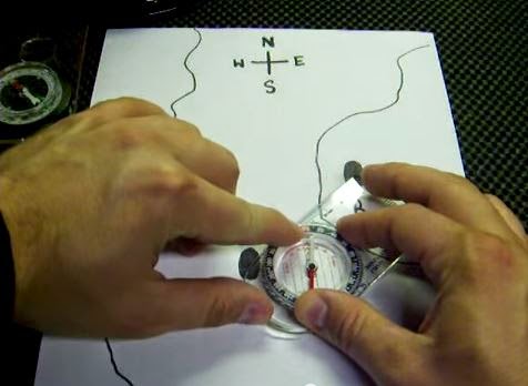
Figure 4. Align the straight edge of the compass between your points, sometimes it's helpful to even draw a line on
you map to indicate your direction of travel. Make sure to the compass facing the correct way. Note the arrow on the
top right of the compass, this should be pointing TOWARDS your direction of travel.

1) Align edge of compass between points A & B, as shown in figure 4.

2) Orient compass dial to map North/True North, as shown in figure 5.

3) Record the bearing closest to the direction-of-travel line on the compass. This will be the bearing you will need to follow to reach your destination.

Figure 5. Orient your compass to your map. Keeping the edge of your compass connecting the two points, turn the dial on the compass towards North on the map. Often times orienteering maps with have grids on them which you can use to help guide your orientation of your compass. This can be done by making the grid parallel to the lines on the inside of your dial. figure 4 shows a close up of the compass and is easier to see the parallel orientation lines.

If you have multiple points to travel to, it is common practice to write down the bearing on your map so you can continue to navigate your points without having to find your bearing at every point. Figure 6 shows the compass on the map with the bearing towards the direction of travel.

4) Keeping the compass at a comfortable chest height (preferably away from any metal objects), turn your body until the red end of the needle is in the red arrow/box on the compass. This position is often referred to as getting "red in the shed."

5) Now facing the same direction, turn the dial to the same bearing you just found.

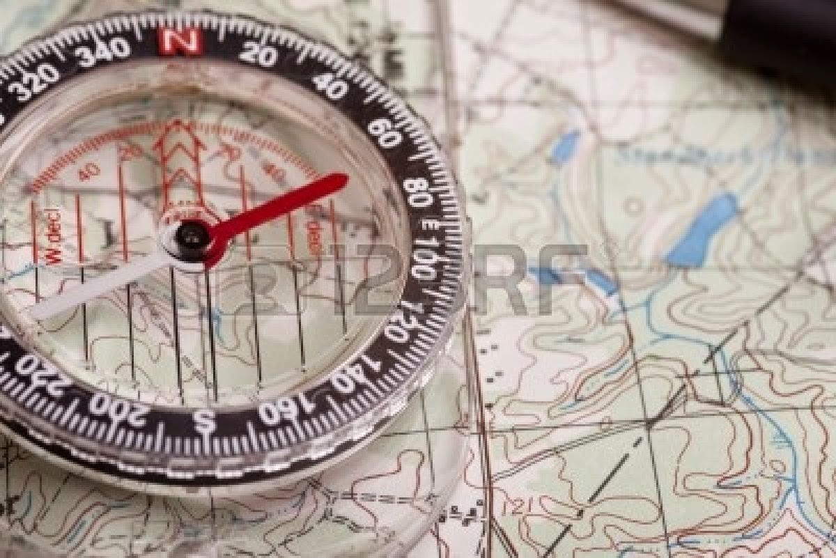
6) To reach your location, all you need to do is keep the red end of the needle in that red box and you will travel along that same line you drew from points A to B. Figure 6 shows a compass oriented to the map. Notice how the lines inside the dial are parallel to the grid lines on the map. This technique is helpful when trying to ensure the compass is oriented as accurately as possible to north on the map.

Figure 6 shows a compass oriented to true north on a topographical map.

The final aspect of navigation will be calculating the distance travel while out in the field. Following the bearing is important, but if you don't know how far you have traveled you will still not know your accurate position without analysis of your map. A rather simple method of keeping track of your distance traveled is called "pace count." As described earlier, an individual's pace count is calculated by walking a standardized distance and remembering how many steps were taken. To lessen the counting and ease the process, only every other step is counted. For example, only count the number of steps you take with your right foot. Once your pace count is determined you can use the number of steps you take to interpolate the distance you have traveled.

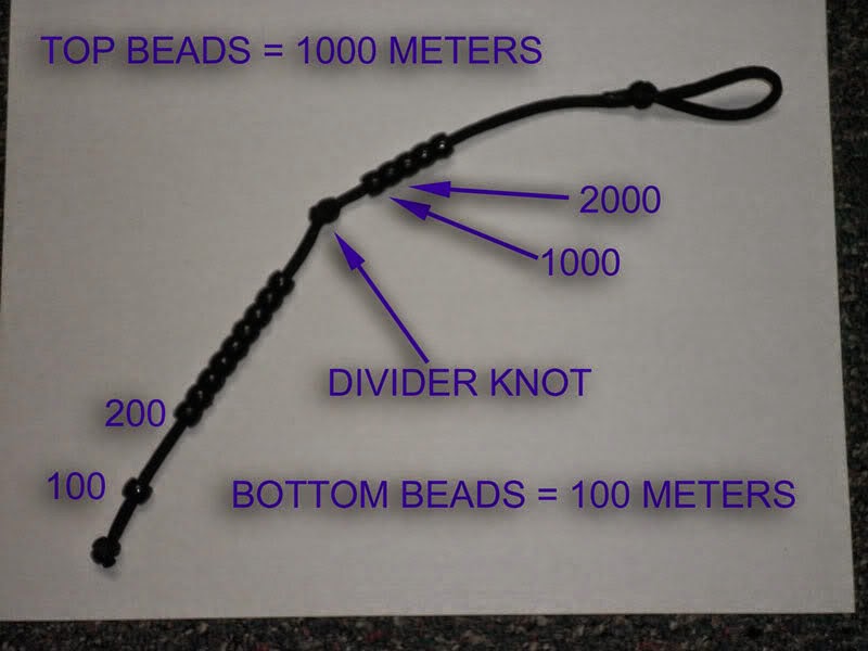
Sometimes long distances between points must be traveled. In order to ensure you do not lose track of your pace count tools or strategies can be involved. One method is to break off a twig every 100 meters and put it in you pocket. There are also cheep tools such as beads on a string, shown in figure 7, which act as a counting mechanism.

Figure 7 shows a cheep tool which can help you remember the number of
steps you have taken between you points. Once you reach your desired
point you would reset the beads to zero.

Discussion

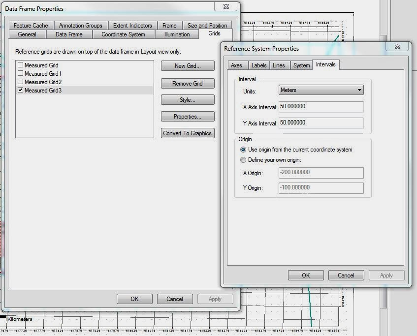
This was a straight forward assignment, but it wasn't without its bumps. I couldn't figure out how to add a grid for the longest time. I knew it was in the data frame properties window under the 'grids' tab, but for some reason when I was creating the grids they would not show up. After some time playing around with the various tabs in the properties menu, looking in the 'Help' files, and trying to add new grids I figured it out. The units were not in meters and the intervals were set much too large to appear on the grid. Figure 8 shows the interface where I had my moment of clarity and fixed the necessary parameters.


Figure 8 The data frame properties menu. Here it is possible to add a grid
in the layout view. For the navigation of the Priory, a 50 meter grid was
decided to be of best fit.

Another topic of debate was how many map elements would be necessary for an effective map. I have a personal fascination with elevation. I knew the DEM would be too much, but the elevation needed to be displayed since it would be an integral part of the navigation. Eventually I chose the 5 meter contour lines to best portray the lay of the land, yet freeing up the map from unnecessary clutter.

Additional map elements could have been added. Knowing where soft boggy areas are, poor footing along slopes, and other such areas would be helpful for navigating. Not all of these elements could be added without the need of a magnifying glass, but if there was a way to display them, navigation in the field could be improved.  However, I have not yet been to the Priory course and lack the first hand experience of the terrain. With this limitation, the contours and the aerial images were the main tools I used and I could not ascertain such fine details from this small of a scale (1:4,500).

Figure 9 shows the final product for the map. A grid at 50 meter intervals was used, as well as contour lines at 5 meter intervals.

Figure 9 Shows the map of the Priory with 5 meter contour intervals, roads, 'no shooting' zones, boundaries for both
point boundaries of the navigation course (yellow polygon), and a boundary for the navigation zone (hollow red square).
NAD 1983 UTM Zone 15N

Conclusion

The effectiveness of the Priory maps will not be known until out in the field. However, based on the tasks mentioned in the write up and the elements included in the map I have confidence the map will serve its purpose. The important component to the map is to make sure the grid can be used effectively to locate the points on the map. Additionally, the grid will be relied on in the field while using pace count, distance, and azimuth to navigate between the points. Until then theory and personal judgment will have to satisfy the requirements until the field testing begins.

EX 4: Conducting a Distance Azimuth Survey

Introduction:

As one of the main goals from the University of Wisconsin - Eau Claire, to graduate as a critical thinker, today's lab was an important variation of that idea. Often times the unexpected can limit your capabilities by having your equipment fail, weather complications, or other unforeseen complications. Without the proper motivation and/or creativity, these problems could delay the survey and waste valuable time. That is why having other tools at your disposal is vital to completing the objectives for whatever project you may be involved with.

Today's project was designed to facilitate creativity and teach the method of distance azimuth, specifically its use in surveying. Given the event that your GPS battery dies in the field, distance azimuth could be used to collect points. As long as the location of your survey point is known, as a reference point, the distance and azimuth--the angle from true north (0°) measured clockwise--can be used to find the relative location of additional points.

Methods:

Magnetic declination, sometimes called magnetic variation, is the angle between magnetic north and true north. Declination is considered positive east of true north and negative when west. Magnetic declination changes over time and with location. Figure 1 shows a map of magnetic declination for the United States in 2010. Magnetic declination for Eau Claire Wisconsin (Latitude: 44.7985°, Longitude: -91.482444°) is -1° 5' West, declination is NEGATIVE.



Figure 1. Created by the National Geophysical Data Center (NOAA).
Magnetic Declination for Eau Claire, WI is negative (-1° 5' West)

Figure 2 Using a tripod for the range finder was an effective method
for dealing with the user error that could have resulted when shifting
from side-to-side during the 1.5 hours it took to find the distance
and azimuth of the trees, signs, and buildings from this central location.

Using distance azimuth is an effective way to collect data; however, this method largely hinges on the use of high accuracy and precision when all the points are calculated from a central location. That is why knowing the exact location of surveyor is of the utmost importance. If this point is off by even a foot, then all the other points collected will have the same error. In addition to knowing the correct position of the surveyor, keeping the location constant is important. If the surveyor is taking steps from side-to-side while collecting data the azimuth with change. Even a eight inches could change the azimuth by a degree or two, and over 100 meters this could result in a much larger error. In short, distance azimuth relies heavily on consistent technique and high accuracy records concerning surveyor position. Figure 2 shows how the group tried to deal with keeping a consistent location for all 100 data points collected as well as a prominent location which could be found on an aerial image (corner of tennis court used to find the lat./long. of the surveyor).

Figure 3 Shows the interface for the Table to Table
Tool. This tool allows the importation of a table
into an existing geodatabase.

After surveying in the field, the rest of the process was focused on creating a feature class of points. This point feature class would represent the objects 'shot' during the survey. The first step was creating a table of the survey in excel. Next, that table had to be imported into a geodatabase (Figure 3 shows the import process). Although the work in the field was carried out as carefully as possible, the values were slightly flawed.

Figure 4 An illustration of Earth's shifting poles. Note the discrepancy between magnetic north and true north
or the "north pole."

Due to the complex processes within the Earth's core, magnetic fields are produced. We use these to navigate with our current day compasses. However, every 200,000-300,000 years the poles switch. This is not an over night event, but a slow fluctuating process. This is

Figure 5 The field calculator was used on the azimuth
field to adjust for the switching of Earth's magnetic poles.
-1° 5' west was the magnetic declination adjustment used
because of the survey location in Eau Claire, WI.

the reason for the previously described phenomena described in Figure 4 with the magnetic declination. For Eau Claire, WI (latitude: 44.802536°, longitude: -91.500164°) the magnetic declination was -1.083333. This value was then used in the field calculator to adjust the azimuth of each angle. Figure 5 shows the equation used to correct for the changing of the poles.

Figure 6 shows the interface for the Bearing Distance to Line
tool. It is important to add the correct fields for the x- and y-
fields. For this survey the latitude (y-field) and longitude
(x-field) at the corner of a tennis court was used.

This was important because the laser was giving the azimuth for magnetic north; and, for surveying true north is desired. True north can be find by adding/subtracting, depending on your location, the magnetic declination from the azimuth. Since the excel table only had fields for ID, distance, and azimuth, the data was still useless. Without a reference point the data had no spatial relationship to the rest of the world. This was corrected by adding x- and y-fields which would represent the latitude and longitude of the reference point for each individual surveyed point. For this study, only one reference point was used. However, in real world examples a clear line of sight will not always be available. If this was the case the x- and y- fields would contain different values depending on the latitude and longitude from which the survey was conducted. In a future study it would be wise to add the spatial location into the excel table during the field work/before importing the table into the geodatabase. That way if there was multiple survey locations the points would already have their own spatial reference point and the risk of error created during the data management phase could be taken out of the process.

Finally the data was in proper form to be used in the Bearing Distance to Line tool (Data Management -Toolbox, Features -toolset). Figure 6  shows the interface for the tool, Figure 7 shows the result of the tool. Note the inputs required of the tool for it to run properly. Now you can have a better understanding of why the table had to be so meticulously prepared before its use.


Figure 7 shows the result of the Bearing Distance to Line
tool. With 100 inputs this feature class has limited use
for analysis. You can see where each line stops; however,
points close to the reference point are difficult to see
where their respective line segments stop. As such, additional
tools must be used before the representation is complete.

Figure 8 shows the interface for the Feature Vertices to Points
tool. Note the help file to the right and the method used for
this feature class, "END." This means a point will be created
at the end off all the vertices, but NOT at the origin/start
of the vertices.

The final step in the exercise was to create a point feature class from the output of the previously used tool, bearing distance to line. This was accomplished with the Feature Vertices to Points tool (Data Management -Toolbox, Features -toolset). Figure 8 shows the interface for the tool, as well as the inputs. Note the option "END" was used to produce this particular feature class. The decision was made because this feature class was going to be used in combination with the output from the bearing distance to line tool. Figure 9 shows the result of the Feature Vertices to Points tool.


Figure 9 shows the final results of the survey. Note
the origin of all the green lines. This is the reference
point were all the data was collected from using the
laser range finder.

Discussion:

Now that the survey and feature classes have been completed, the analysis of accuracy can be completed. Looking at Figure 9 every yellow point should have its correlating tree, parking sign, house, or bridge support pillar. When the points don't match up, a question should be asked. Why isn't there a feature under that point? There are many reasons for this. The image used might be temporally inaccurate. To get a better estimate of when this image was taken, an analysis of the surrounding area was needed. If you are familiar with the University of Wisconsin-Eau Claire you would quickly recognize some discrepancies. There has been a lot of construction as of late with one student center being demolished, another being built just to the South, and a new education building close by. Only the beginning stages of the student center are visible in this aerial. The official date of construction started on March 7th, 2011. As you can see by Figure 10, construction has just started to begin. Only the preparatory stages have occurred at the time of this photo. Suggesting the date to be around early spring time. Other reasons could stem from different projections used, distortions during the mosaicking of images, or user error in the field.

Figure 10 Construction on the new Davie's Center began March 7th, 2011. You can already see a trailer and
disturbed ground. Figure 11 shows the Davie's building during mid-construction.

Figure 11 The W.R. Davies Student Center took just over
2 years to build. The aerial photo above shows the building
during mid-construction, likely during mid-summer of 2012
using the color of the leaves as clues, and the knowledge
that the previous building was demolished in August of 2012.
The old building is still standing in Figure 11.

Conclusion:

In order to understand distance and azimuth, many aspects of surveying had to be researched. Phenomena such as the shifting of Earth's poles, magnetic declination, operation of a compass, etc. Although each piece of the lab was not individually a keystone piece of information. Collectively they created a deep understanding being the principles of distance and azimuth. At the end of the lab I felt very confident I knew what I was doing and I could lead others in the field where distance and azimuth could be put to use.

EX 3: Using Unmanned Aerial Systems (UAS) to Solve Geospatial Problems

Introduction:

This lab three member group effort to better understand Unmanned Aerial Systems (UAS) by talking five real world problems. The problems required critical thinking and research. As most the students in the class were unframiliar with UASs, often called UAVs (Unmanned Aerial Vehicles), research into the components of a UAS was a must to understand how the drone could be used, ultimately, in the solution to the geospatial problems created for this exercise.


UAV Overview

An Unmanned Aerial Vehicle (UAV) is an aircraft that has the capability of autonomous flight, without a pilot in control. Amateur UAVs are non-military and non-commercial. They typically fly under “recreational” exceptions to FAA regulations on UAVs, so long as the pilots/programmers keep them within tight limits on altitude (below 400 feet above ground level for recreational use) and distance. Usually the UAV is controlled manually by Radio Control (RC) at take-off and landing, and switched into GPS-guided autonomous mode only at a safe altitude.

FAA UAS Regulations

• Operator must have a Civil UAS certificate
• Shows airworthiness proficiency
• Operator must have a Public UAS permit
• Enabling the operator to fly in civil air space
• NOTE: Current law prohibits the flying of UAS over airports, cities, and private air space.

What do you need to make a UAV?

1) RC plane, multicopter, or helicopter. Can buy them ready to fly, including autopilot.

2) Autopilot, such as APM 2.6

• APM 2.6 autopilot: the electronics, including twin processors, gyros, accelerometers, pressure sensors, GPS and more. Retail $179.
• APM 2 is an open source, Arduino-compatible, pro-quality autopilot.
• APM 2 supports any kind of vehicle with a one-click change of code.
• Available codes include:
• ArduPlane (fixed wing)
• ArduCopter (rotary wing)
• ArduRover (ground vehicles)
• Provides an entire UAV control system with scriptable missions with:
• 3D waypoints
• In-flight uploading of commands
• Powerful ground station software.

3) Mission Planner software: Desktop software that lets you manage APM and plan missions, along with being a powerful ground station during flights and helping you analyze mission logs afterwards.

• Autopilot software:
• Arduplane: for fixed-wing aircraft
• Features included in arduplane
• Return to launch with a flick of your RC toggle switch or a mouse click in the graphical Ground Station
• Unlimited 3D GPS waypoints
• Built-in camera control
• Fully-scriptable missions
• One-click software load, and easy point-and-click configuration in the powerful Mission Planner. NO programming required.
• Replay recorded missions and analyze all the data with a graphing interface
• Supports two-way telemetry with Xbee wireless modules.
• Point-and-click waypoint entry or real-time mission commands while the UAV is in the air
• Fly with a joystick or gamepad via your PC-no need for RC control
• Built-in failsafe will return the aircraft in case of radio failure
• Arducopter: for rotary-wing aircraft
• ArduRover: for any ground- or water-based vehicle

4) “Payload,” such as a digital camera, video transmission equipment, or other optional sensors.

 

Fixed wing craft:

Budget of craft - $1000 with: telemetry kit (wireless communication), 3 batteries, and the OSD/FPV kit (enable the viewing of live streaming video). http://store.3drobotics.com/products/3DR-ARF-APM:Plane

Advantages -

More forgiving (than rotary craft) in the event of mechanical failure and/or pilot error do to their natural ability to glide without power. Can carry greater payloads for longer distances on less power. Have longer flight time than the helicopters (Gas: around 10 hours, Electric: around 45-60 minutes).

 

Disadvantages -

Cannot hover over one spot, meaning they cannot provide the same level of precision, for point specific scenarios. Cannot perform vertical takeoff 

Helicopter – Single Rotary Craft

About:

• 1-2 blades to generate lift
• Maintain directional control by varying blade pitch
• Gas or electric
• Medium range

They are safer if you can have a separate motor battery and radio battery. This helps prevent radio and APM:Copter power loss when the motor battery drains)***Hint: Disconnecting the power to the motor is one easy method to be sure that the motor will not turn while you are configuring the Arducopter system.
Advantages

• Vertical liftoff with ability to hover.
• This allows for increased detail in hard to reach situations.
• Real-time feedback
• Can carry various sensors:
• Day
• Low-light
• Night vision
• IR sensors
• Strong, fast and efficient
• Some can be weatherized

 

Disadvantages

• Range: limited on payload
• Fuel Type and flight time:
• Electric: 20min - 90min
• Gas: 4-5 hours
• More limited flight time and payload capacity when compared to a fixed-wing craft

commando http://www.uavsi.uk.com/docs/UAVSI_COMMANDO_Heli-UAV_Brochure.pdf

sniper http://www.uavsi.uk.com/docs/UAVSI_SNIPER_Heli-UAV_Brochure.pdf

Pulse Aerospace:http://pulseaero.com/products/vapor-helicopter-uas.php      www.rotomotion.com

Multicopter

About:

• Excellent for surveying smaller areas at high levels of detail.
• Can hover in place when greater detail and zoom is required.
• Utilizes differential thrust management of independent motor units to provide lift and directional control.
• Simple mechanical design, large degree of design flexibility.
• Allows many options for mounting payload.
• Carries a decent payload in strong wind conditions.
• Multiple arms decreases the risk of serious injury.
• Battery life ~20 minutes max.
• Typically, more arms = less battery life

Require computer control for stable flight, if computer isn’t working the copter isn’t flying.
The copter compensates for gusts of wind by tilting automatically against the direction of the disturbance.

Multicopter system: http://copter.ardupilot.com/wp-content/uploads/sites/2/2013/07/copter-diagram.png

The Quadcopter is simplest, most popular, and most reliable. If you are inexperienced, start small. The quadcopers are easier to fly, light, tough, relatively safe, and survive mishaps well.

Multicopters are highly stressed systems and require that all components match compatibility:
Projected weight, performance, flight time, and payload require balancing to achieve good results.
Frame size, weight, power requirements, and payload are important to consider

Good starter: http://traxxas.com/products/models/heli/6208qr1
Highly recommended system complete with pre-mission software: http://store.3drobotics.com/products/iris

Scenarios:

#1 (Brielle ) A military testing range is having problems engaging in conducting its training exercises due to the presence of desert tortoises. They currently spend millions of dollars doing ground based surveys to find their burrows. They want to know if you, as the geographer can find a better solution with UAS.
Questions to ask:
Where are the turtles?
herbivores, feed on grasses/wildflowers/cactus pads (http://www.defenders.org/desert-tortoise/basic-facts)
97% of borrows associated with shrub vegetation (FS)

Deep burrows under large/near large boulders (FS)

95% of life spent in burrows (https://www.desertusa.com/reptiles/desert-tortoise.html)

The presence of soil suitable for digging burrows is a limiting factor to Desert Tortoise distribution (desert usa). Soil that crumbles easily during digging and is firm enough to resist collapse (http://www.fs.fed.us/database/feis/animals/reptile/goag/all.html#Soil)

Commonly use sites with sandy loam soils with varying amounts of gravel and clay (FS). Avoid sands (FS).

Dig basins to collect rain water (desert usa)

What sensors can locate the burrows/turtles?

How big are they? 3-6ft deep (defenders).

How are they capable of being located? temp? Vegetation

When turtles move, how far? Do they stay in one burrow?

Stay in burrows in torpor from November-February (defenders)

Most active in Spring (defenders)

Is burrow count accurate to turtle numbers? Single tortoise may have dozens of borrows across range (desert usa)

Do turtles return to same burrow? no/possible

Where are the closest natural areas?

How large is the testing range?

Are there multispectral satellite images available?

Are training exercises continual or scheduled for certain time spans?

How often are the exercises conducted

How often do the tortoise surveys need to be done

Possible solutions:

Landsat-Resolution isn’t fine (60m)

NIR scanner for vegetation detection Landsat 8 ban; Landsat(4 or 5) band4

Thermal image for burrow entrances? Landsat(4 or 5) band 6; Landsat 8 band 10/11

Soil maps- Landsat(4 or 5) band 5 or 6

Fixed wing craft-large area

NIR scanner-vegetation detection

Thermal imager-burrow entrances

Short-wave infrared scanner-soil signatures

Duration: due to large area, longer duration; gas powered more reliable

#2 (Tim) A power line company spends lots of money on a helicopter company monitoring and fixing problems on their line. One of the biggest costs is the helicopter having to fly up to these things just to see if there is a problem with the tower. Another issue is the cost of just figuring how to get to the things from the closest airport.

Questions to ask:

How often do problems occur along the power lines? How much does it cost to get the helicopter out to inspect the line? Are the lines accessible to ground crews to get close enough quickly enough? What type of area are the power lines in, populated or rural?

Possible solutions:

A multi-copter would be a good option to perform this task. A ground crew with the multicopter would get close enough to the power lines that they wish to examine in order to use a multicopter The UAV multicopter should be installed with a high quality camera and should be able to operate at a relatively low noise level to prevent disturbing wildlife or cattle that may be in the area. It would also be advantageous to have some way for the copter to detect changes in the electrical field around it so it could detect anything that may be wrong with the power lines.

The multicopter at the link below is one of the standard and typical multicopters used for this type of work. It has a high payload capacity (3kg) for high definition imagery, has it’s rotors covered for safety when flying near power lines, is equipped with excellent crash/accident avoidance technology such as its “coming home” function, is very stable when holding position for excellent imagery, and comes with some of the best pre-mission programming. It will cost around $30,000 per multicopter but this will pay off in the long run when considering that the company is paying thousands upon thousands of dollars EACH time the helicopter has to go out to check the power lines. It’s a cheap start up cost but will pay off in the end, as this is a very reliable model.

http://www.aibotix.com/features.html

http://www.hoverspective.com/en/products/aibotix-x-6-en

http://www.aibotix.com/inspection-of-high-voltage-power-lines.html

It may be a good idea to have a UAV helicopter along as well, this way, if a power line needs to be looked at rapidly due to some sort of emergency, the helicopter drone can be launched from further away due to it’s longer range. The same considerations regarding weight, noise level, image quality, and maneuverability would need to be taken into consideration for the helicopter drone as for the multicopter.

The Black Eagle designed by steady copter is a solid option that can hover within 5 meters of the power line and has a 3kg capacity. It will cost around $10,000. This start up cost is less than that of the Aibot x6 multicopter above so this may be a better option if the company decides that it would be too difficult to get close to the power lines.

http://www.steadicopter.com/Page.aspx?ID=128286576

http://www.youtube.com/watch?v=51pEXkkL3A0

http://www.steadicopter.com/Page.aspx?ID=306457996

Both the Aibot multicopter and the Black Eagle helicopter UAVs would be good options for this job. I think that recommending both to the company and pointing out the benefits/drawbacks of both would be a good option.

#3 (Tim) A pineapple plantation has about 8000 acres, and they want you to give them an idea of where they have vegetation that is not healthy, as well as help them out with when might be a good time to harvest.

Questions to ask:

What type of area is the pineapple plantation in?

What is currently being done to assess these problems?

Possible solution:

UAV helicopter equipped with NIR camera sensor which will detect higher reflectance of healthy vegetation. This UAS would require a pre mission software that would allow it to track and cover the whole field recording data spatially. Ideally this would be done during the day when there is the highest amount of NIR reflection.

A gas helicopter would be a good option for this, perhaps the Sniper with a NIR camera mounted on it. This is because the field is too large for the flight time of a multi-copter but needs the focus and maneuverability of a helicopter. http://www.uavsi.uk.com/docs/UAVSI_SNIPER_Heli-UAV_Brochure.pdf

The near infrared camera can be used to tell whether vegetation is healthy or not. There is a high range of difference in the NIR (720nm-1300nm) reflectance of healthy vegetation and unhealthy vegetation. Healthy vegetation reflects significantly more NIR waves. This means that in NIR images the healthy vegetation will appear more prominently than the unhealthy vegetation. http://flightriot.com/nir-and-vegetation/

Pineapple plants are read to harvest when they are in the late stages of their development. This means that they have over 1/3 of their peel as a yellow color but they haven’t lost all of their green yet.

http://homeguides.sfgate.com/pineapple-ripe-ready-picked-plant-54066.html

NIR reflection has been tested to see whether or not it can be used to detect ripeness of a plant, as the plant gets riper, the NIR tends to decrease. This fact combined with the fact that when pineapples are ready to harvest they shouldn’t be ripe yet and shouldn’t be harvested until their skin is 1/3 yellow and 2/3 green can help determine the best time to harvest the pineapple. Using a multi-spectral approach with both visible wavelengths to try and determine color and NIR wavelengths to determine health and whether the plant is ready to harvest.

 #4 (Jacob) An oil pipeline running through the Niger River delta is showing some signs of leaking. This is impacting both agriculture and loss of revenue to the company.

Questions to ask:

How big is the range of possible leakage in the pipe?

Will there be any restricted areas to avoid?

Risk of fire hazard?

Will the UAS be flying over any populated areas?

What time of year will the surveying take place?

Possible solution:

Because this is dealing with such a large area you will need a UAS with a large antenna which will allow for longer flight time. Also, you will be sensing expansive areas, without the need for high definition, so the precision brought on by a multicopter is not needed. The best type of craft for this mission would be a gas powered fixed-wing craft. Given the fact that they are recruiting you from half a world away, it is fair to assume that the $1,000 price tag for an intermediate plane is not to high.

The main sensor on the plane would be a small thermal imaging camera, to fly autonomously along the pipeline, just after sunset, to record the thermal images of the ground, from which one can deduce the thermal heat capacity of the ground, around the pipeline.
 

Just after sunset, there will be a drop in temperature, just as there will be an increase after sunrise, and one can interpret the thermal images, to estimate the heat capacity of the ground. If these images are taken once a day, one should be able to detect leakage from any of the pipeline joints because of the change in heat capacity of the ground given the event of a leaking leaking joint. 

One should have a time dependent view of the changes. This suggested approach rests on the heat capacity of the oil and the ground being different from that of the ground alone.

What is needed to accomplish this?

• Construct a 3D computer based thermal model of the buried pipeline and surrounding soil.
• Heat capacity of properly functioning pipeline
• Thermal conductivity data. For the materials (land, water, vegetation, etc.) in the immediate areas to the pipeline.
• Would also need to monitor the temperatures at various depths along the pipeline. To determine the heating effect of the sun’s rays during day time. The rate of cooling. As a function of depth and location along the pipeline, during the night time.
• With a combination of the computer model and measurement information, one would relate the minimum sensitivity of a thermal imaging system to the size of the leak that could be detected. The measurement information would also be used to determine the best time to perform the thermal imaging, likely, just after sunset.

Barnard Microsystems. A Suggested Way to Detect Oil Leakage. http://www.barnardmicrosystems.com/UAV/pipeline_monitoring/detect_oil_leakage.html

 #5 (Jacob) A mining company wants to get a better idea of the volume they remove each week. They don’t have the money for LiDAR, but want to engage in 3D analysis (Hint: look up point cloud)

Questions to ask:

What is your budget for the project?

How expansive is your mining operation?

Is your mine an open pit mine?

Possible solution using  Photosynth (for PC):

• Install the Photosynth application
• Install Image Composite Editor
• Use SynthExport to extract the point cloud as well as camera parameter data of your synth on Photosynth.
• Supported Point Cloud formats
• OBJ (no vertex colors stored)
• Polygon file format (ASCII and binary)
• VRML
• X3D
• Use a product like Meshlab to generate a mesh surface from the point cloud.

 

Once you have the point cloud ArcMap could do the rest, but “Meshlab” is a free and open source software which might be better if you are assuming the mining company has small budget and in that case, possibly you don’t have access to ArcMap.

Once you have created a 3D surface, say in ArcMap, you could use the “Surface Volume” tool (3D Analyst Extension).
The Surface Volume tool calculates the area and volume of a raster or TIN surface above or below a given reference plane.

Using this tool you could set the plane at a control depth; which, would stay the same each week. Then you would calculate the volume of the ground each week. Theoretically the volume of that ground would decrease each week as the ground is excavated. This change in volume would be the amount of material mined each week.

Take an abundance of photos with sufficient overlap (>60%)

Photosynth picks out identifiables points that are common to multiple photos, then uses the different distances, angles and relative sizes of the points in the images to work out the 3D arrangement of the actual points on the real object, which it generates a point cloud from. http://diydrones.com/forum/topics/making-digital-elevations

The number of photos taken from a fixed-wing plane may not be enough to get a dense mesh.

Using a kite might actually work better.
Perk of using a Kite:
You can collect data as long as the wind is blowing
Much cheaper than buying the small UAV and all the systems that go along with it.
Imagery must have at least 60% in-track overlap and should have at least 40% cross-track/orthogonal overlap. Imagery must be shot in sequence. Imagery includes overlap.

Sources used in research:
Drone Mapper, Hints & Tips
Making Inexpensive Digital Elevation models